MATLAB練習(xí)例子七(數(shù)據(jù)處理)
返回
》 load count.dat
》 [n,p] = size(count)
n =
24
p =
3
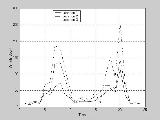
》 t = 1:n;
》 set(0,'defaultaxeslinestyleorder','-|--|-.')
》 set(0,'defaultaxescolororder',[0 0 0])
》 plot(t,count), legend('Location 1','Location 2','Location 3',0)
》 plot(t,count), legend('Location 1','Location 2','Location 3',0) xlable('Time'),ylabel('Vehicle Count'), grid on
??? cation 3',0) xlable
|
演算子、カンマ、またはセミコロンが見つかりません
》 plot(t,count), legend('Location 1','Location 2','Location 3',0) xlabel('Time'),ylabel('Vehicle Count'), grid on
??? cation 3',0) xlabel
|
演算子、カンマ、またはセミコロンが見つかりません
》 plot(t,count), legend('Location 1','Location 2','Location 3',0),xlabel('Time'),ylabel('Vehicle Count'), grid on
》 plot(t,count), legend('Location 1','Location 2','Location 3',0),xlabel('Time'),ylabel('Vehicle Count'), grid on
》 type count.dat
11 11 9
7 13 11
14 17 20
11 13 9
43 51 69
38 46 76
61 132 186
75 135 180
38 88 115
28 36 55
12 12 14
18 27 30
18 19 29
17 15 18
19 36 48
32 47 10
42 65 92
57 66 151
44 55 90
114 145 257
35 58 68
11 12 15
13 9 15
10 9 7
 基本數(shù)據(jù)分析
》 load count.dat
》 mx = max(count)
mx =
114 145 257
》 mu = mean(count)
mu =
32.0000 46.5417 65.5833
》 sigma = std(count)
sigma =
25.3703 41.4057 68.0281
》 [mx,indx] = min(count)
mx =
7 9 7
indx =
2 23 24
》 [n,p] =size(count)
n =
24
p =
3
》 e = ones(n,1)
e =
1
1
1
1
1
1
1
1
1
1
1
1
1
1
1
1
1
1
1
1
1
1
1
1
》 x = count - e*mu
x =
-21.0000 -35.5417 -56.5833
-25.0000 -33.5417 -54.5833
-18.0000 -29.5417 -45.5833
-21.0000 -33.5417 -56.5833
11.0000 4.4583 3.4167
6.0000 -0.5417 10.4167
29.0000 85.4583 120.4167
43.0000 88.4583 114.4167
6.0000 41.4583 49.4167
-4.0000 -10.5417 -10.5833
-20.0000 -34.5417 -51.5833
-14.0000 -19.5417 -35.5833
-14.0000 -27.5417 -36.5833
-15.0000 -31.5417 -47.5833
-13.0000 -10.5417 -17.5833
0 0.4583 -55.5833
10.0000 18.4583 26.4167
25.0000 19.4583 85.4167
12.0000 8.4583 24.4167
82.0000 98.4583 191.4167
3.0000 11.4583 2.4167
-21.0000 -34.5417 -50.5833
-19.0000 -37.5417 -50.5833
-22.0000 -37.5417 -58.5833
》 min(count(:))
ans =
7
協(xié)方差和對射變模
》 cov(count(:,1))
ans =
643.6522
》 corrcoef(count)
ans =
1.0000 0.9331 0.9599
0.9331 1.0000 0.9553
0.9599 0.9553 1.0000
》 A = [9 -2 3 0 1 5 4];
》 diff(A)
ans =
-11 5 -3 1 4 -1
數(shù)據(jù)預(yù)處理(Data Preprocessing)
》 mu = mean(count)
mu =
32.0000 46.5417 65.5833
》 sigma = std(count)
sigma =
25.3703 41.4057 68.0281
》 [n,p] = size(count)
n =
24
p =
3
》 outliers = abs(count - mu(ones(n,1),:)) > 3*sigma(ones(n,1),:);
》 nout = sum(outliers)
nout =
1 0 0
》 count(any(outliers'),:) = [];
回歸分析
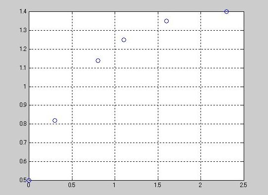
》 t = [0 .3 .8 1.1 1.6 2.3]';
》 y = [0.5 0.82 1.14 1.25 1.35 1.40]';
》 plot(t,y,'o'),grid on
基本數(shù)據(jù)分析
》 load count.dat
》 mx = max(count)
mx =
114 145 257
》 mu = mean(count)
mu =
32.0000 46.5417 65.5833
》 sigma = std(count)
sigma =
25.3703 41.4057 68.0281
》 [mx,indx] = min(count)
mx =
7 9 7
indx =
2 23 24
》 [n,p] =size(count)
n =
24
p =
3
》 e = ones(n,1)
e =
1
1
1
1
1
1
1
1
1
1
1
1
1
1
1
1
1
1
1
1
1
1
1
1
》 x = count - e*mu
x =
-21.0000 -35.5417 -56.5833
-25.0000 -33.5417 -54.5833
-18.0000 -29.5417 -45.5833
-21.0000 -33.5417 -56.5833
11.0000 4.4583 3.4167
6.0000 -0.5417 10.4167
29.0000 85.4583 120.4167
43.0000 88.4583 114.4167
6.0000 41.4583 49.4167
-4.0000 -10.5417 -10.5833
-20.0000 -34.5417 -51.5833
-14.0000 -19.5417 -35.5833
-14.0000 -27.5417 -36.5833
-15.0000 -31.5417 -47.5833
-13.0000 -10.5417 -17.5833
0 0.4583 -55.5833
10.0000 18.4583 26.4167
25.0000 19.4583 85.4167
12.0000 8.4583 24.4167
82.0000 98.4583 191.4167
3.0000 11.4583 2.4167
-21.0000 -34.5417 -50.5833
-19.0000 -37.5417 -50.5833
-22.0000 -37.5417 -58.5833
》 min(count(:))
ans =
7
協(xié)方差和對射變模
》 cov(count(:,1))
ans =
643.6522
》 corrcoef(count)
ans =
1.0000 0.9331 0.9599
0.9331 1.0000 0.9553
0.9599 0.9553 1.0000
》 A = [9 -2 3 0 1 5 4];
》 diff(A)
ans =
-11 5 -3 1 4 -1
數(shù)據(jù)預(yù)處理(Data Preprocessing)
》 mu = mean(count)
mu =
32.0000 46.5417 65.5833
》 sigma = std(count)
sigma =
25.3703 41.4057 68.0281
》 [n,p] = size(count)
n =
24
p =
3
》 outliers = abs(count - mu(ones(n,1),:)) > 3*sigma(ones(n,1),:);
》 nout = sum(outliers)
nout =
1 0 0
》 count(any(outliers'),:) = [];
回歸分析
》 t = [0 .3 .8 1.1 1.6 2.3]';
》 y = [0.5 0.82 1.14 1.25 1.35 1.40]';
》 plot(t,y,'o'),grid on
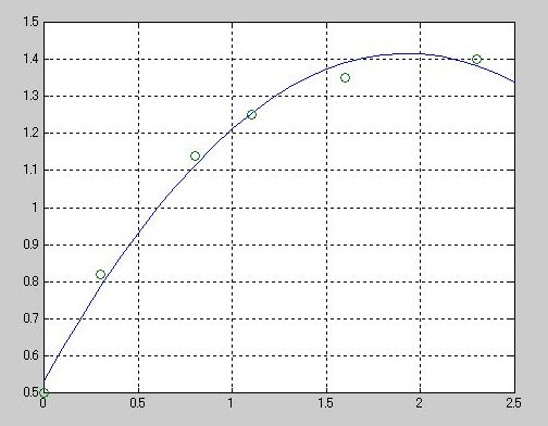
 多項(xiàng)式回歸分析
》 X = [ones(size(t)) t t.^2
]
X =
1.0000 0 0
1.0000 0.3000 0.0900
1.0000 0.8000 0.6400
1.0000 1.1000 1.2100
1.0000 1.6000 2.5600
1.0000 2.3000 5.2900
》 a = X\y
a =
0.5318
0.9191
-0.2387
》 T = (0:0.1:2.5)';
》 Y = [ones(size(T)) T T.^2]*a;
》 plot(T,Y,'-',t,y,'o'), grid on
多項(xiàng)式回歸分析
》 X = [ones(size(t)) t t.^2
]
X =
1.0000 0 0
1.0000 0.3000 0.0900
1.0000 0.8000 0.6400
1.0000 1.1000 1.2100
1.0000 1.6000 2.5600
1.0000 2.3000 5.2900
》 a = X\y
a =
0.5318
0.9191
-0.2387
》 T = (0:0.1:2.5)';
》 Y = [ones(size(T)) T T.^2]*a;
》 plot(T,Y,'-',t,y,'o'), grid on
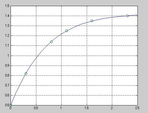
 線性回歸分析
》 X = [ones(size(t)) exp(- t) t.*exp(- t)];
》 a = X\y
a =
1.3974
-0.8988
0.4097
》 Y = [ones(size(T)) exp(- T) T.exp(- T)]*a;
??? Attempt to reference field of non-structure array 'T'.
》 T = (0:0.1:2.5)';
》 Y = [ones(size(T)) exp(- T) T.exp(- T)]*a;
??? Attempt to reference field of non-structure array 'T'.
》 T = (0:0.1:2.5)';
》 Y = [ones(size(T)) exp(- T) T.exp(- T)]*a;
??? Attempt to reference field of non-structure array 'T'.
》 Y = [ones(size(t)) exp(- t) T.exp(- t)]*a;
??? Attempt to reference field of non-structure array 'T'.
》 Y = [ones(size(t)) exp(- t) t.exp(- t)]*a;
??? Attempt to reference field of non-structure array 't'.
》 Y = [ones(size(T)) exp(- T) T.*exp(- T)]*a;
》 plot(T,Y,'-',t,y,'o'), grid on
線性回歸分析
》 X = [ones(size(t)) exp(- t) t.*exp(- t)];
》 a = X\y
a =
1.3974
-0.8988
0.4097
》 Y = [ones(size(T)) exp(- T) T.exp(- T)]*a;
??? Attempt to reference field of non-structure array 'T'.
》 T = (0:0.1:2.5)';
》 Y = [ones(size(T)) exp(- T) T.exp(- T)]*a;
??? Attempt to reference field of non-structure array 'T'.
》 T = (0:0.1:2.5)';
》 Y = [ones(size(T)) exp(- T) T.exp(- T)]*a;
??? Attempt to reference field of non-structure array 'T'.
》 Y = [ones(size(t)) exp(- t) T.exp(- t)]*a;
??? Attempt to reference field of non-structure array 'T'.
》 Y = [ones(size(t)) exp(- t) t.exp(- t)]*a;
??? Attempt to reference field of non-structure array 't'.
》 Y = [ones(size(T)) exp(- T) T.*exp(- T)]*a;
》 plot(T,Y,'-',t,y,'o'), grid on
 線性回歸分析
》 x1 = [.2 .5 .6 .8 1.0 1.1]';
》 x2 = [.1 .3 .4 .9 1.1 1.4]';
》 y = [.17 .26 .28 .23 .27 .24]';
》 X = [ones(size(xa) x1 x2];
??? = [ones(size(xa) x1
|
関數(shù)の參照が正しくありません。","、または ")" が足りません
》 X = [ones(size(x1)) x1 x2];
》 a = X\y
a =
0.1018
0.4844
-0.2847
》 Y = X*a;
》 MaxErr = max(abs(Y - y)
??? rr = max(abs(Y - y)
|
関數(shù)の參照が正しくありません。","、または ")" が足りません
》 MaxErr = max(abs(Y - y))
MaxErr =
0.0038
》 plot(T,Y,'-' t,y,'o'), grid on
??? plot(T,Y,'-' t
|
関數(shù)の參照が正しくありません。","、または ")" が足りません
》 T = (0:0.1:2.5)';
》 X
X =
1.0000 0.2000 0.1000
1.0000 0.5000 0.3000
1.0000 0.6000 0.4000
1.0000 0.8000 0.9000
1.0000 1.0000 1.1000
1.0000 1.1000 1.4000
》 plot(T,Y,'-',t,y,'o'), grid on
??? エラー: ==> plot
ベクトルは同じ長さである必要があります.
》 X = [ones(size(x1)) x1 x2];
》 a = X\y
a =
0.1018
0.4844
-0.2847
》 Y = X*a
Y =
0.1703
0.2586
0.2786
0.2332
0.2731
0.2362
》 plot(T,Y,'-',t,y,'o', grid on
??? -',t,y,'o', grid on
|
関數(shù)の參照が正しくありません。","、または ")" が足りません
》 plot(T,Y,'-',t,y,'o'), grid on
??? エラー: ==> plot
ベクトルは同じ長さである必要があります.
》 load census
》 p = polyfit(cdate,pop,4)
Warning: Matrix is close to singular or badly scaled.
Results may be inaccurate. RCOND = 5.429790e-020.
> In C:\MAT\toolbox\matlab\polyfun\polyfit.m at line 52
p =
1.0e+005 *
0.0000 -0.0000 0.0000 -0.0126 6.0020
》 sdate = (cdate -mean(cdate))./std(cdate)
sdate =
-1.6116
-1.4505
-1.2893
-1.1282
-0.9670
-0.8058
-0.6447
-0.4835
-0.3223
-0.1612
0
0.1612
0.3223
0.4835
0.6447
0.8058
0.9670
1.1282
1.2893
1.4505
1.6116
》 p = polyfit(sdate,pop,4)
p =
0.7047 0.9210 23.4706 73.8598 62.2285
》 pop4 = polyval(p,sdate);
》 plot(cdate,pop4,'-',cdate,pop,'+'), grid on
線性回歸分析
》 x1 = [.2 .5 .6 .8 1.0 1.1]';
》 x2 = [.1 .3 .4 .9 1.1 1.4]';
》 y = [.17 .26 .28 .23 .27 .24]';
》 X = [ones(size(xa) x1 x2];
??? = [ones(size(xa) x1
|
関數(shù)の參照が正しくありません。","、または ")" が足りません
》 X = [ones(size(x1)) x1 x2];
》 a = X\y
a =
0.1018
0.4844
-0.2847
》 Y = X*a;
》 MaxErr = max(abs(Y - y)
??? rr = max(abs(Y - y)
|
関數(shù)の參照が正しくありません。","、または ")" が足りません
》 MaxErr = max(abs(Y - y))
MaxErr =
0.0038
》 plot(T,Y,'-' t,y,'o'), grid on
??? plot(T,Y,'-' t
|
関數(shù)の參照が正しくありません。","、または ")" が足りません
》 T = (0:0.1:2.5)';
》 X
X =
1.0000 0.2000 0.1000
1.0000 0.5000 0.3000
1.0000 0.6000 0.4000
1.0000 0.8000 0.9000
1.0000 1.0000 1.1000
1.0000 1.1000 1.4000
》 plot(T,Y,'-',t,y,'o'), grid on
??? エラー: ==> plot
ベクトルは同じ長さである必要があります.
》 X = [ones(size(x1)) x1 x2];
》 a = X\y
a =
0.1018
0.4844
-0.2847
》 Y = X*a
Y =
0.1703
0.2586
0.2786
0.2332
0.2731
0.2362
》 plot(T,Y,'-',t,y,'o', grid on
??? -',t,y,'o', grid on
|
関數(shù)の參照が正しくありません。","、または ")" が足りません
》 plot(T,Y,'-',t,y,'o'), grid on
??? エラー: ==> plot
ベクトルは同じ長さである必要があります.
》 load census
》 p = polyfit(cdate,pop,4)
Warning: Matrix is close to singular or badly scaled.
Results may be inaccurate. RCOND = 5.429790e-020.
> In C:\MAT\toolbox\matlab\polyfun\polyfit.m at line 52
p =
1.0e+005 *
0.0000 -0.0000 0.0000 -0.0126 6.0020
》 sdate = (cdate -mean(cdate))./std(cdate)
sdate =
-1.6116
-1.4505
-1.2893
-1.1282
-0.9670
-0.8058
-0.6447
-0.4835
-0.3223
-0.1612
0
0.1612
0.3223
0.4835
0.6447
0.8058
0.9670
1.1282
1.2893
1.4505
1.6116
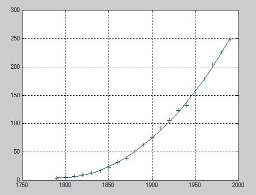
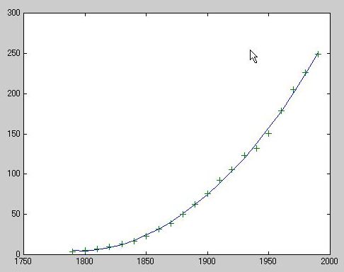
》 p = polyfit(sdate,pop,4)
p =
0.7047 0.9210 23.4706 73.8598 62.2285
》 pop4 = polyval(p,sdate);
》 plot(cdate,pop4,'-',cdate,pop,'+'), grid on
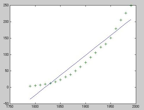
 》 p1 = polyfit(sdate,pop,1);
》 pop1 = polyval(p1,sdate);
》 plot(cdate,pop1,'-',cdate,pop,'+')
》 p1 = polyfit(sdate,pop,1);
》 pop1 = polyval(p1,sdate);
》 plot(cdate,pop1,'-',cdate,pop,'+')
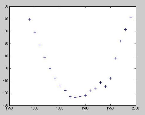
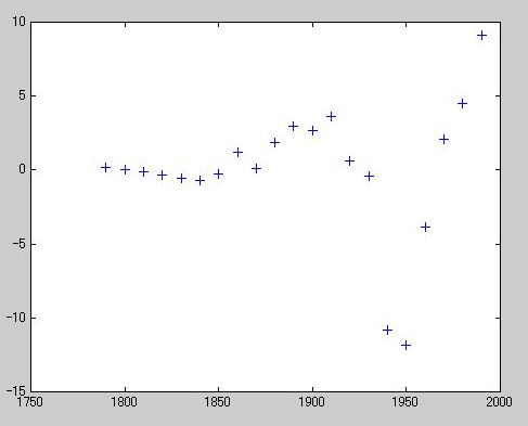
 》 res1 = pop - pop1;
》 figure, plot(cdate,res1,'+')
》 res1 = pop - pop1;
》 figure, plot(cdate,res1,'+')
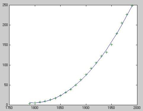
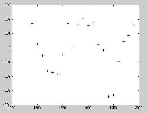
 》 p = polyfit(sdate,pop,2);
》 pop2 = polyval(p,sdate);
》 plot(cdate,pop2,'-',cdate,pop,'+')
》 p = polyfit(sdate,pop,2);
》 pop2 = polyval(p,sdate);
》 plot(cdate,pop2,'-',cdate,pop,'+')
 》 res2 = pop - pop2;
》 figure, plot(cdate,res2,'+')
》 res2 = pop - pop2;
》 figure, plot(cdate,res2,'+')
 》 p = polyfit(sdate,pop,4);
》 pop4 = polyval(p,sdate);
》 plot(cdate,pop4,'-',cdate,pop,'+')
》 p = polyfit(sdate,pop,4);
》 pop4 = polyval(p,sdate);
》 plot(cdate,pop4,'-',cdate,pop,'+')
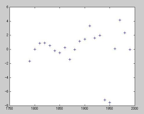
 》 res4 = pop - pop4;
》 figure,plot(cdate,res4,'+')
<img src="res32.jpg">
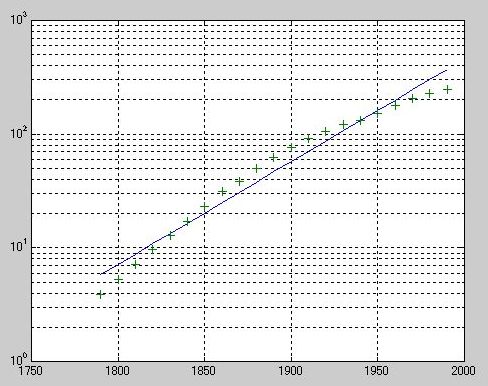
》 logp1 = polyfit(sdate,log10(pop),1);
》 logpred1 = 10.^polyval(logp1,sdate);
》 semilogy(cdate,logpred1,'-',cdate,pop,'+');
》 grid on
》 res4 = pop - pop4;
》 figure,plot(cdate,res4,'+')
<img src="res32.jpg">
》 logp1 = polyfit(sdate,log10(pop),1);
》 logpred1 = 10.^polyval(logp1,sdate);
》 semilogy(cdate,logpred1,'-',cdate,pop,'+');
》 grid on
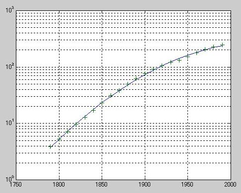
 》 logp2 = polyfit(sdate,log10(pop),2);
》 logpred2 = 10.^polyval(logp2,sdate);
》 semilogy(cdate,logpred2,'-',cdate,pop,'+'); grid on
》 logp2 = polyfit(sdate,log10(pop),2);
》 logpred2 = 10.^polyval(logp2,sdate);
》 semilogy(cdate,logpred2,'-',cdate,pop,'+'); grid on
 》 logres2 = log10(pop) - polyval(logp2,sdate);
》 plot(cdate,logres2,'+')
》 logres2 = log10(pop) - polyval(logp2,sdate);
》 plot(cdate,logres2,'+')
 》 r = pop - 10.^(polyval(logp2,sdate));
》 plot(cdate,r,'+')
》 r = pop - 10.^(polyval(logp2,sdate));
》 plot(cdate,r,'+')
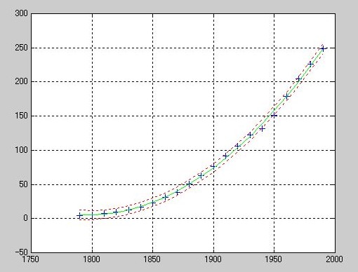
 plot(cdate,pop,'+',cdate,pop2,'g-',cdate,pop2+2*del2,'r:',cdate,pop2-2*del2,'r:'), grid on
 Fast Fourier Transform
》 x = [4 3 7 -9 1 0 0 0]';
》 y = fft(x)
y =
6.0000
11.4853 - 2.7574i
-2.0000 -12.0000i
-5.4853 +11.2426i
18.0000
-5.4853 -11.2426i
-2.0000 +12.0000i
11.4853 + 2.7574i
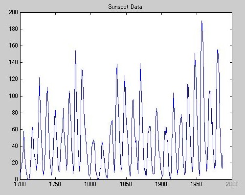
》 load sunspot.dat
》 year = sunspot(:,1);
》 wolfer = sunspot(:,2);
》 plot(year,wolfer)
》 title('Sunspot Data')
Fast Fourier Transform
》 x = [4 3 7 -9 1 0 0 0]';
》 y = fft(x)
y =
6.0000
11.4853 - 2.7574i
-2.0000 -12.0000i
-5.4853 +11.2426i
18.0000
-5.4853 -11.2426i
-2.0000 +12.0000i
11.4853 + 2.7574i
》 load sunspot.dat
》 year = sunspot(:,1);
》 wolfer = sunspot(:,2);
》 plot(year,wolfer)
》 title('Sunspot Data')
 》 Y = fft(wolfer);
》 N = length(Y);
》 Y(1) = [];
》 power = abs(Y(1:N/2)).^2;
》 nyquist = 1/2;
》 freq = (1:N/2)/(N/2)*nyquist;
》 plot(freq,power),grid on
》 xlabel('cycles/year')
》 title('Periodogram')
》 Y = fft(wolfer);
》 N = length(Y);
》 Y(1) = [];
》 power = abs(Y(1:N/2)).^2;
》 nyquist = 1/2;
》 freq = (1:N/2)/(N/2)*nyquist;
》 plot(freq,power),grid on
》 xlabel('cycles/year')
》 title('Periodogram')
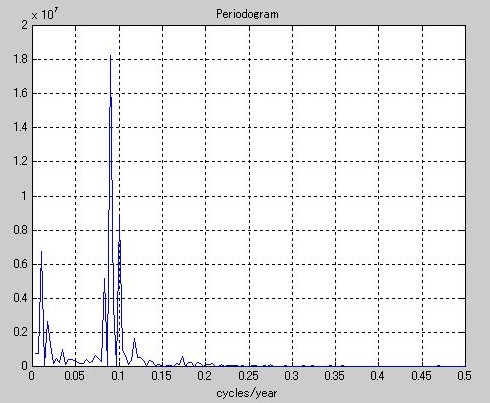 》 period = 1./freq;
》 plot(period,power), axis([0 40 0 2e7]), grid on
》 ylabel('Power')
》 xlabel('Period(Years/Cycle)')
》 period = 1./freq;
》 plot(period,power), axis([0 40 0 2e7]), grid on
》 ylabel('Power')
》 xlabel('Period(Years/Cycle)')
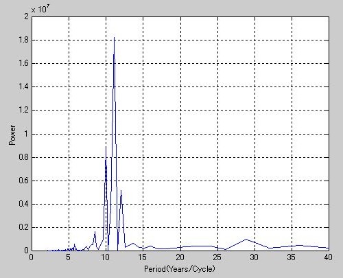 》 [mp index] = max(power);
》 period(index)
ans =
11.0769
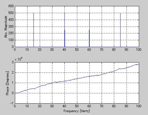
》 t = 0:1/100:10-1/100;
》 x = sin(2*pi*15*t) + sin(2*pi*40*t);
》 y = fft(x);
》 m = abs(y);
》 p = unwrap)angle(y));
??? p = unwrap)
|
演算子、カンマ、またはセミコロンが見つかりません
》 p = unwrap(angle(y));
》 f = (0:length(y)-1)'*100/length(y);
》 subplot(2,1,1), plot(f,m),
》 ylabel('Abs. Magnitude'), grid on
》 subplot(2,1,2), plot(f,p*180/pi)
》 ylabel('Phase [Degrees]'), grid on
》 xlabel('Frequency [Hertz]')
》 [mp index] = max(power);
》 period(index)
ans =
11.0769
》 t = 0:1/100:10-1/100;
》 x = sin(2*pi*15*t) + sin(2*pi*40*t);
》 y = fft(x);
》 m = abs(y);
》 p = unwrap)angle(y));
??? p = unwrap)
|
演算子、カンマ、またはセミコロンが見つかりません
》 p = unwrap(angle(y));
》 f = (0:length(y)-1)'*100/length(y);
》 subplot(2,1,1), plot(f,m),
》 ylabel('Abs. Magnitude'), grid on
》 subplot(2,1,2), plot(f,p*180/pi)
》 ylabel('Phase [Degrees]'), grid on
》 xlabel('Frequency [Hertz]')
返回
潮安县|
环江|
石柱|
嘉荫县|
吉水县|
安平县|
嘉祥县|
芷江|
高邮市|
巧家县|
永登县|
建昌县|
保德县|
蚌埠市|
南京市|
奉新县|
清苑县|
防城港市|
龙陵县|
濮阳市|
通山县|
祁门县|
辽中县|
元氏县|
连平县|
定州市|
舞阳县|
蓬安县|
铁岭县|
广水市|
绥江县|
怀柔区|
井冈山市|
图木舒克市|
大英县|
扎鲁特旗|
九寨沟县|
民丰县|
东辽县|
西乌|
右玉县|